Computation Of Future Intrinsic Value Of TATA MOTORS LTD Stock

Introduction

This is the construction of the discounted cash flow methodology in order to estimate the intrinsic value of TATA Motors Ltd stock after 5 years that is in the year 2030. In order to predict the financial statement elements for the next five years from the year 2025, I have put in use, Gemini AI. The values predicted by the model are included in this case. After retrieving the future financial values of the elements of the financial statements, I proceeded with the DCF modelling process. 

Note: I put in use the Gordon Growth method in order to calculate terminal value as part of the DCF process.

Future values:

Income Statement:

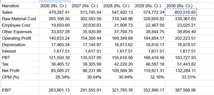
Cash Flow Statement:

Balance Sheet:

Financial prediction Model:

The driver based financial model forecasted sales value from a small set of explicit well thought out assumptions rather than historical statistical relationships.

1. The sales prediction methodology

the sales figure is the most important input, as all other figures are projected as a percentage of this number.

the model uses a two factor growth rate approach:

 Sales Growth=(1+Volume/Demand Growth)×(1+Price/Realization Growth)

 This method provides better nuance than a simple single growth rate, allowing us to model market expansion (volume) and brand strength (pricing) separately.

A. GDP Proxy Growth (The Volume/Demand Driver)

Role: This driver acts as a proxy for the expected volume increase or market expansion for Tata Motors, reflecting economic activity in its core markets (India and key overseas markets for JLR).

Assumption: The initial growth is aggressive (8% in 2026) reflecting the strong turnaround at JLR and the domestic EV push, before gradually normalizing to a long-term growth rate (5% by 2029-2030).

Impact: This translates directly into how many more cars and commercial vehicles the company is expected to sell each year.

B. Competitor Impact (The Price/Realization Driver)

Role: This driver represents the company's ability to increase the average price per unit or shift its product mix to higher-value vehicles. This is often called price realization.

Assumption: The model assumes a slight, constant positive impact of 0.5% each year.

Rationale: This suggests that Tata Motors has improving pricing power, perhaps due to:

• The successful premiumization of the JLR brand.

• Increased sales of high-margin electric vehicles (EVs) in the domestic market.

• Higher-margin commercial vehicle sales.

Impact: This ensures the projected revenue grows not just because of volume, but also due to improved profitability per vehicle sold.

Cost & Operational Efficiency Drivers

These drivers determine the Operating Profit (EBIT) margin. They are modelled to transition from the historical ratio towards a pre-defined industry-standard target, reflecting expected efficiency gains.

Driver	Role in Model	Assumption Trend
Raw_Material_Cost_Pct_Target (COGS)	Models Cost of Goods Sold as a percentage of Sales.	Target of 61%. The model assumes improved procurement and manufacturing efficiency over time.
Employee_Cost_Pct_Target	Models payroll and related expenses as a percentage of Sales.	Target of 4.0%. Reflects a stable, efficient workforce relative to growing sales.
Other_Exp_Pct_Target	Models General & Administrative (G&A) overheads.	Target of 7%. Assumes operational overhead remains tightly controlled.

Capital Expenditure and Tax Drivers

Driver	Role in Model	Assumption Trend
Capex_Pct_of_Sales	Determines the annual investment in property, plant, and equipment.	Declines from 5.5% to 3.5%. This is critical: it reflects the assumption that large platform investments (like those for new EVs) will be completed, and future CapEx will normalize to maintenance and incremental upgrades.
Tax_Rate	Directly calculates tax expense on Profit Before Tax (PBT).	Starts at 30% and settles at 28%. This reflects the current Indian corporate tax regime.

E. Working Capital Drivers

These variables ensure the Balance Sheet and Cash Flow Statement are properly linked by projecting current assets based on sales velocity.

Driver	Metric Used	Assumption Trend
Debtor_Days	Days Sales Outstanding (DSO)	Declines from 15 to 11 days. This assumes the company gets paid faster by customers, freeing up cash.
Inventory_Days	Days Inventory Outstanding (DIO)	Declines from 40 to 32 days. This assumes the company improves its supply chain and reduces the time products sit on the shelf.

Process of the Discounted Cash Flow Model:

The following are the steps involved in the computation of the DCF  model.

After predicting the future values:

1) Calculate Free Cash Flows:

By using the mathematical formula:

2) Calculate Weighted Average Cost of Capital (WACC):

In order to calculate the WACC value, one need to arrive at cost of equity

Following is the process of calculating cost of equity:

Then one can calculate WACC Value:

3) Forecast Explicit Period Cash Flows:

Discount the FCFs for each forecast year:

4) Estimate Terminal value

Perpetual Growth (Gordon Growth):

5) Calculate Enterprise Value:

Calculate the enterprise value by employing the following formula:

6) Get Equity value and Share Value

Key assumptions:

Growth & Operations (FCFF Drivers)

Revenue growth:

 Key Assumption: 

starts high at 8.5% combined growth due to expected strong JLR performance and domestic EV leadership, then declines to 5.5% by 2030. 

Rational: High valuation driver: a small change here has the largest impact on the final FCFF and therefore the enterprise value.

Operating Margins: improving efficiency: raw material, employee and other costs are modelled to improve moving from current ratios towards industry best-practice targets (Raw material settling at 61%,=.

Rational: profitability: this ensures that as sales grow, the operating profit grows faster, leading to higher net operating profit after tax (NOPAT)

Capital expenditure: declining investment: capex as a percentage of sales is modelled to decrease sharply from 5.5% to 3.5%.

cash flow booster: this assumes the heavy investment cycle that is the new EV Platforms and is concluding, freeing up more cash flow for investors.

Working capital: efficiency gains: debtors days and inventory days are modelled to decline steadily.

sources of cash: this create a working capital release adding to the FCFF each year.

Tax Rate: stable tax regime: the average tax rate is assumed to settle at 28% from an initial 30%.

predictability: assumes no maker changes in corporate tax policy and that the company is fully utilizing available deductions

Findings:

The ultimate outcome of the DCF model predicted the intrinsic share value of TATA Motors LTD for the year 2030

The intrinsic value of TATA Motors Ltd for the year 2030 : ₹4502.43/-

Disclaimer: This Discounted Cash Flow (DCF) model is based on assumptions and forward-looking estimates, and is not a guarantee or reliable predictor of future stock value. Actual market conditions, company performance, and other real-world factors will cause the stock's value to be dynamic and subject to constant change. Furthermore, I am not registered or authorized by the Securities and Exchange Board of India (SEBI) or any other regulatory body to provide investment advice. This model and any related discussion should not be construed as financial or investment advice.